Energy data engineering / forecast impact
Regional Energy Data Lake
A three-layer data lake for asking a narrow market question with messy, versioned inputs: when a weather or generation forecast is wrong, what relationship does the error have with the next observed electricity price?
Research question
Do forecast errors line up with market outcomes after the obvious time patterns are accounted for?
The project does not try to forecast prices with a black-box model. It first makes the data lineage explicit, then asks whether forecast error is associated with day-ahead price, price volatility, and negative-price probability. That distinction matters because the same realized market outcome is observed against multiple forecast vintages.
End-to-end process
From raw source files to one panel I can rerun
- A
1. Keep the source vintages
Store downloaded files, checksums, manifests, and ingestion batches in Bronze so a result can be traced back to a source file.
- B
2. Make timestamps explicit
Parse UTC timestamps, keep source resolution, standardize column names and units, and preserve rejected or missing records for review.
- C
3. Join realized and forecast weather
For each forecast run, align the realized weather outcome with the forecast available at that run time rather than using a later revision.
- D
4. Build the Gold impact panel
Create one analysis-ready table with day-ahead price, renewable regime, weather errors, generation forecast errors, and residual load.
- E
5. Estimate conditional relationships
Fit zone, hour, and date fixed-effects models with standard errors two-way clustered by valid time and forecast run.
- F
6. State what the design cannot identify
Treat the estimates as conditional associations. The current sample is one month, the weather coverage is sparse, and market outcomes repeat across vintages.
Visual evidence
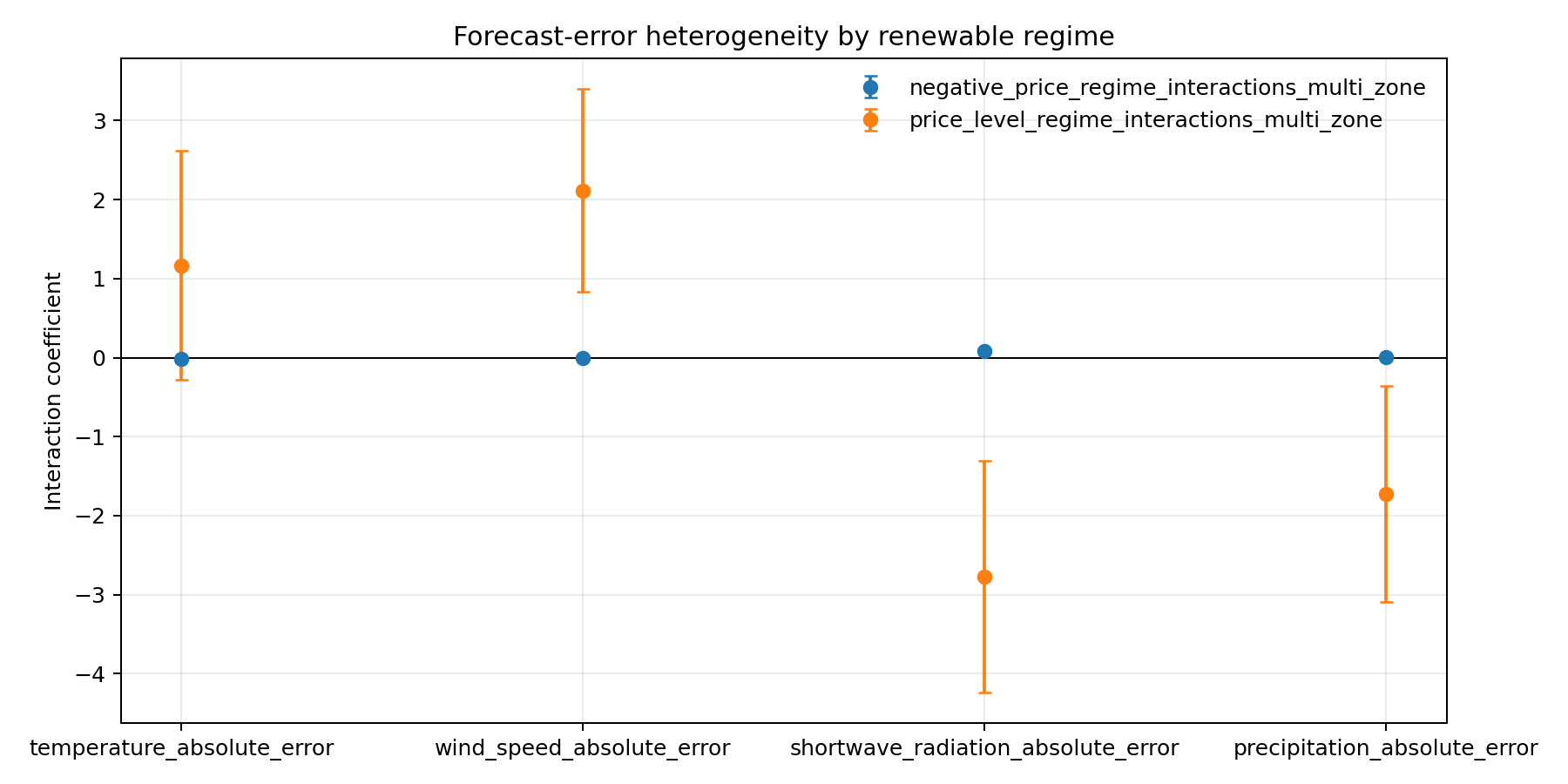
The zone split is part of the result
Descriptive results
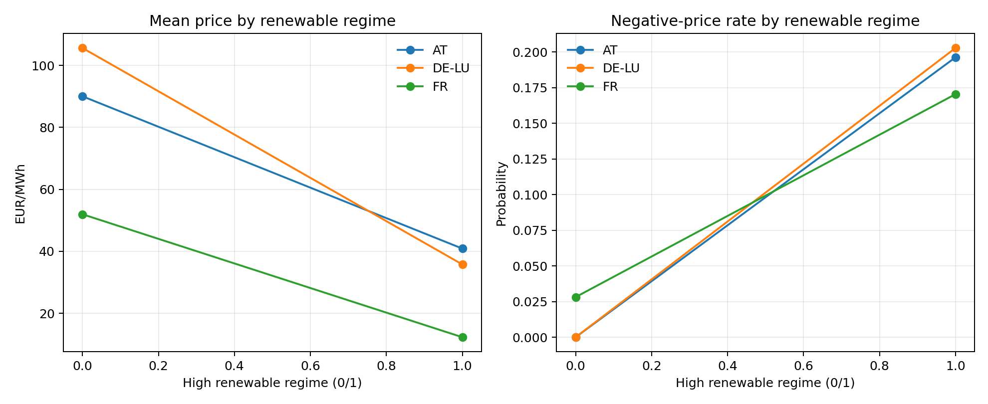
High-renewable hours are cheaper in every zone
The regime split is defined inside each zone. It is a descriptive comparison, not a causal estimate, but it gives a useful check before fitting the fixed-effects models.
| Zone | Low-renewable mean €/MWh | High-renewable mean €/MWh | High-regime negative-price rate |
|---|---|---|---|
| DE-LU | 105.63 | 35.75 | 20.28% |
| AT | 90.03 | 40.87 | 19.62% |
| FR | 51.95 | 12.26 | 17.04% |
Model specification
A simple model with uncertainty treated seriously
The main price model includes bidding-zone, UTC hour, and valid-date fixed effects. Continuous predictors are standardized within zone. Standard errors are two-way clustered by valid time and forecast run, with 30 forecast runs setting the smallest cluster count.
| Outcome | Rows | R² | Forecast-run clusters | Model type |
|---|---|---|---|---|
| Day-ahead price | 21,510 | 0.8372 | 30 | Price level |
| Price with regime interactions | 21,510 | 0.8398 | 30 | Price level |
| 24-hour price volatility | 21,480 | 0.6237 | 30 | Volatility |
| Negative-price indicator | 21,510 | 0.5335 | 30 | Binary outcome |
R² is descriptive fit, not out-of-sample forecasting accuracy. Repeated market outcomes across vintages are the reason the forecast-run dimension is part of the inference design.
Selected coefficients
What the model says, conditionally
| Predictor | Coefficient | Clustered p-value | Reading |
|---|---|---|---|
| Actual residual load | +19.05 | <0.001 | Higher residual load is associated with higher price. |
| Solar forecast error | −2.27 | <0.001 | The standardized error has a negative price association. |
| Wind-onshore forecast error | −2.62 | <0.001 | The standardized error has a negative price association. |
| Temperature absolute error | −1.44 | <0.001 | Temperature error is associated with lower price in this panel. |
The coefficient signs are consistent with a market where residual load pushes prices up while positive renewable-generation forecast errors coincide with lower prices. These are conditional associations in the current panel; they should not be read as causal effects of changing the forecast.
Final takeaway
The point is being able to trace the result back to the source
The useful part of this project is the connection between versioned ingestion and statistical interpretation. Bronze preserves what arrived, Silver makes the source differences inspectable, and Gold gives the model one reproducible panel. The current result is a clear next step rather than a finished claim: extend the vintage history, add more representative weather points, and test whether the zone-specific relationships survive across seasons.
Read the code and reports on GitHub